Dask: A Parallel Computing Library for Scalable Data Processing

Introduction

In the realm of data processing, handling large datasets efficiently is a critical challenge. While Pandas has been the default choice for many Python users, it struggles with scalability, particularly when working with datasets larger than available memory. Enter Dask—a parallel computing library designed to extend the capabilities of Pandas by enabling seamless scaling across cores and even distributed systems.

Dask’s familiar Pandas-like interface, combined with its ability to process data in chunks and utilize parallelism, makes it an ideal choice for tackling large-scale data problems without extensive code rewrites. This blog delves into how Dask works, its advantages, and a practical example showcasing its performance benefits.

Efficient Data Processing with Dask

Handling large datasets poses unique challenges in memory and processing power. Dask simplifies this process by:

• Distributing data processing across multiple CPU cores or machines.

• Breaking datasets into smaller chunks for out-of-core computation.

• Retaining a familiar API for users transitioning from Pandas.

We’ll demonstrate how Dask can handle a real-world dataset and compare its performance to Pandas in key operations like file reading, filtering, and processing.

How Dask Works

Dask operates by creating a computation graph and deferring execution until explicitly triggered. Here’s a breakdown:

1. Setup a Computation:

Dask builds a computation graph representing the tasks and their dependencies, including data loading and transformations.

2. Execute the Computation:

Execution begins when .compute() is called. Tasks are processed in parallel across CPU resources, optimizing performance.

Example: Processing a Large CSV File with Dask

Objective:

Efficiently process a large CSV file containing loan-level data. We’ll compare Dask’s performance against Pandas in tasks like reading, filtering, and aggregating data.

Step 1: Environment Setup

To initialize Dask for parallel processing, first import the necessary libraries: dask.dataframe as dd, Client from dask.distributed, and psutil. Then, set up the Dask client by creating an instance with Client(n_workers=4).

Step 2: Reading the Data

To read a large CSV file into a Dask DataFrame and measure the time taken, import the time library, record the start time with time.time(), load the file using dd.read_csv('large_file.csv'), display the number of rows and a preview with df.head(), and compute the read time by subtracting the start time from the current time.

Step 3: Filtering the Data

Filter rows where WireAmount > 100 using filtered_df = df[df['WireAmount'] > 100], compute the result with filtered_df.compute(), and optionally monitor memory usage.

Step 4: Aggregating the Data

To compute the mean WireAmount from the filtered dataset, calculate it using mean_value = filtered_df['WireAmount'].mean().compute() and print the result with print(f"Mean WireAmount: {mean_value}").

import dask.dataframe as dd
import time
import psutil
from dask.distributed import Client
from dask.diagnostics import Profiler, ResourceProfiler

# Function to get current memory usage
def memory_in_mb():
    process = psutil.Process()
    mem = process.memory_info().rss  # Get memory usage in bytes
    return mem / (1024 ** 2)  # Convert to MB

# Function to get current CPU usage
def cpu_usage_percent():
    return psutil.cpu_percent(interval=1)

def main():
    # Start Dask Client
    client = Client(n_workers=4)  # Increase workers as needed

    # File path
    file_path = '/home/gowthami/Downloads/big_file.csv'

    # Measure the read time
    start_time = time.time()
    df_dask = dd.read_csv(file_path)  # Dask reads the file and creates a Dask DataFrame
    read_time = time.time() - start_time
    print(f"Total rows read: {df_dask.shape[0].compute()}")  # Print total rows
    print("Preview of the first few rows:")
    print(df_dask.head())  # Print preview of Dask DataFrame

    # Measure initial memory usage
    initial_memory = memory_in_mb()

    # Start profiling
    with Profiler() as prof:
        with ResourceProfiler() as resource_prof:
            total_start_time = time.time()
            # Total processing start time
            total_start_time = time.time()

start_time = time.time()
filtered_dask = df_dask[df_dask['WireAmount'] > 100]  # Define filtering
filtered_dask = filtered_dask.compute()  # Compute the result
filter_time = time.time() - start_time

# Measure memory usage after filtering
memory_after_filtering = memory_in_mb()

# Example processing: Compute the mean of a numeric column
start_time = time.time()
mean_value_dask = filtered_dask['WireAmount'].mean()  # Calculate mean
processing_time_dask = time.time() - start_time

# Measure memory usage after mean calculation
memory_after_processing = memory_in_mb()

# Total processing time
total_processing_time = time.time() - total_start_time

# Measure CPU usage during processing
cpu_usage = cpu_usage_percent()

# Print results
print(f"Dask Read Time: {read_time:.4f} seconds")
print(f"Dask Filter Time: {filter_time:.4f} seconds")
print(f"Dask Processing Time: {processing_time_dask:.4f} seconds")
print(f"Total Processing Time: {total_processing_time:.4f} seconds")
print(f"CPU Usage During Processing: {cpu_usage:.2f}%")
print(f"Initial Memory Usage: {initial_memory:.2f} MB")
print(f"Memory Usage After Filtering: {memory_after_filtering:.2f} MB")
print(f"Memory Usage After Processing: {memory_after_processing:.2f} MB")

# Print profiling results
print(prof.results)
print(resource_prof.results)

if __name__ == '__main__':
    main()

Observations

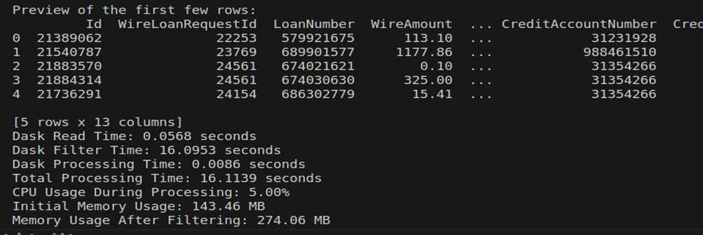
• Dask (2.4GB file): Efficient in reading, filtering, and aggregating data while utilizing minimal memory.

• Pandas (2.4GB file): Handles tasks but faces memory constraints with larger files.

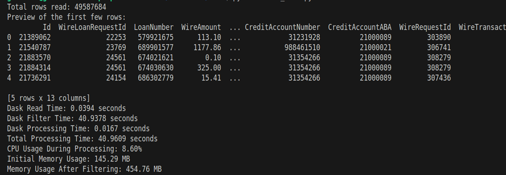
• Dask (6GB file): Processes seamlessly due to chunking and parallelism.

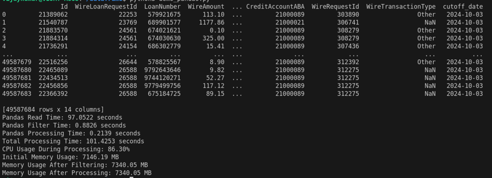
• Pandas (6GB file): Process takes longer time, faces memory constraints, or even encounters memory errors.

Here is the output looks like when I processed 2.4GB file using dask:

Here is the output looks like when I processed 2.4GB file using pandas:

Now observe the difference when I processed the 6GB file  using Dask.

When I processed the 6GB file  using Pandas.

Why Dask Excels with Large Datasets

• Parallel Processing: Utilizes multiple CPU cores for faster execution.

• Out-of-Core Computation: Reads and processes data in chunks, avoiding memory overload.

• Lazy Evaluation: Builds a computation graph and executes only on demand.

• Optimized Data Handling: Uses efficient columnar storage formats.

Advantages of Dask

1. Scalable Memory Usage: Dask’s chunking mechanism allows it to process datasets larger than available memory. Instead of loading the entire dataset, it processes data in manageable chunks, minimizing memory overload and reducing system crashes.

2. Parallel Computing: Dask can execute computations across multiple CPU cores or even clusters of machines, significantly reducing processing time for large datasets. Its task scheduler ensures optimal distribution and coordination of tasks.

3. Familiar API: Designed to resemble the Pandas API, Dask requires minimal changes to existing Pandas-based codebases. Functions like read_csv, groupby, and mean have equivalent Dask implementations, simplifying the transition.

4. Lazy Evaluation: Dask defers computation until .compute() is called, enabling users to build complex pipelines without immediately executing them. This lazy approach minimizes intermediate memory usage and optimizes execution plans.

5. Distributed System Compatibility: Beyond single-machine parallelism, Dask scales seamlessly to distributed clusters, making it a versatile tool for large-scale data engineering and machine learning tasks.

Limitations of Dask

1. Overhead of Parallelism: While Dask excels in parallel processing, the coordination and communication overhead can outweigh benefits for smaller datasets or simple tasks. In such cases, Pandas’ single-threaded execution may be faster and more efficient.

2. Partial API Compatibility: Dask’s API mirrors much of Pandas but is not a complete replica. Some Pandas features, such as in-place operations or advanced indexing, are not available. Users may need to convert Dask DataFrames back to Pandas for certain tasks, potentially introducing inefficiencies.

3. Performance Tuning Requirements: Achieving optimal performance with Dask often requires fine-tuning parameters such as chunk size and the number of workers. Improper configuration can lead to suboptimal performance or increased memory consumption.

4. Complex Debugging: Debugging parallel or distributed code can be challenging. Errors in Dask workflows may stem from its lazy evaluation model or the distributed nature of tasks, making it harder to trace and resolve issues compared to Pandas.

Conclusion

Dask is a transformative library for scaling data processing tasks beyond Pandas' limitations. It shines in scenarios involving large datasets or parallel processing requirements. While it may not replace Pandas for simpler tasks, it is a robust solution for professionals needing efficient, scalable workflows.

Transitioning to Dask involves minimal effort, making it a valuable addition to any data professional’s toolkit. Whether processing local files or distributed systems, Dask delivers unparalleled performance and flexibility.