Handling large datasets can feel overwhelming, especially when you're faced with endless rows of data and complex information. At our company, we faced these challenges head-on until we discovered AWS Athena. Athena transformed the way we handle massive datasets by simplifying the querying process without the hassle of managing servers or dealing with complex infrastructure. In this article, I’ll Walk you through how AWS Athena has revolutionized our approach to data analysis. We’ll explore how it leverages SQL to make working with big data straightforward and efficient. If you’ve ever struggled with managing large datasets and are looking for a practical solution, you’re in the right place.
Efficient Data Storage and Querying
Through our experiences, we found that two key strategies significantly enhanced our performance with Athena: partitioning data and using columnar storage formats like Parquet. These methods have dramatically reduced our query times and improved our data analysis efficiency. Here’s a closer look at how we’ve implemented these strategies:
Data Organization for Partitioning and Parquet
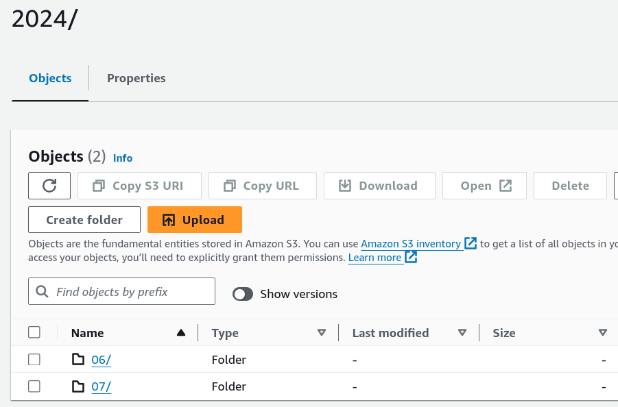
Organize your data in S3 for efficient querying:
s3://your-bucket/your-data/
├── year=2023/
│ ├── month=01/
│ │ ├── day=01/
│ │ │ └── data-file
│ │ └── day=02/
│ └── month=02/
└── year=2024/
└── month=01/
└── day=01/
Preprocessing Data for Optimal Performance
Before importing datasets into AWS Glue and Athena, preprocessing is essential to ensure consistency and efficiency. This involves handling mixed data types, adding date columns for partitioning, and converting files to a format suitable for Athena.
Note: The following steps are optional based on the data and requirements. Use them according to your requirements.
1. Handling Mixed Data Types
To address columns with mixed data types, standardize them to the most common type using the following code snippet:
def determine_majority_type(series):
    # get the types of all non-null values
    types = series.dropna().apply(type)
    # count the occurrences of each type
    type_counts = types.value_counts()
2. Adding Date Columns for Partitioning
To facilitate partitioning, add additional columns for year, month, and day:
def add_date_columns_to_csv(file_path):
    try:
        # read the CSV file
        df = pd.read_csv(file_path)
3. Converting CSV to Parquet Format
For optimized storage and querying, convert CSV files to Parquet format:
def detect_and_convert_mixed_types(df):
    for col in df.columns:
        # detect mixed types in the column
        if df[col].apply(type).nunique() > 1:
4. Concatenating Multiple CSV Files
To consolidate multiple CSV files into one for Parquet conversion:
def read_and_concatenate_csv_files(directory):
    all_dfs = []

    # recursively search for CSV files in the directory
Step-by-Step Guide to Managing Datasets with AWS Glue and Athena
1. Place Your Source Dataset in S3
Upload your source dataset to an S3 bucket. This will serve as the storage location for AWS Glue to access and catalog your data. Proper organization within the bucket facilitates easier data management and access.

2. Create a Crawler in AWS Glue
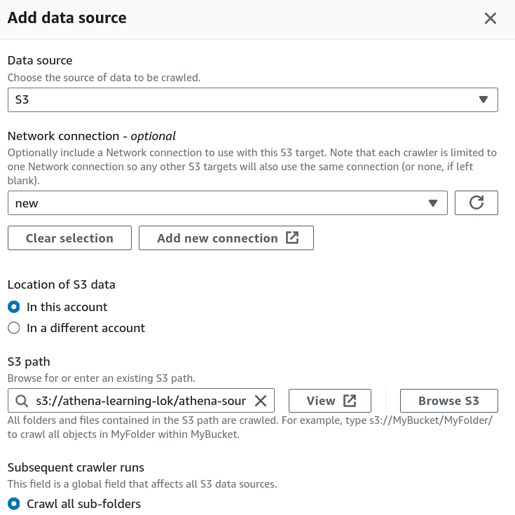
In the AWS Glue console, create a new crawler to catalog your data and make it queryable with Athena.
- Specify Your S3 Bucket: Set the S3 bucket path as the data source in the crawler configuration.
- IAM Role: Assign an IAM role with the necessary permissions to access your S3 bucket and Glue Data Catalog.

3. Set Up the Glue Database
Create a new database in the AWS Glue Data Catalog where your CSV data will be stored. This database acts as a container for your tables.
- Database Creation: Go to the AWS Glue Data Catalog section and create a new database.
- Crawler Output Configuration: Specify this database for storing the table metadata and optionally provide a prefix for your table names.
4. Configure Crawler Schedule
Set the crawler schedule to keep your data catalog up to date:
- Hourly
- Daily
- Weekly
- Monthly
- On-Demand
Scheduling the crawler ensures data will be updated to our table, if any updates to existing data or adding of new files etc.
5. Run the Crawler
Initiate the crawler by clicking the "Run Crawler" button in the Glue console. The crawler will analyze your data, determine optimal data types for each column, and create a table in the Glue Data Catalog.
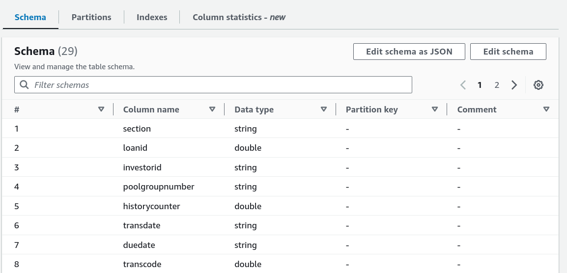
6. Review and Edit the Table Schema
Post-crawler, review and modify the table schema:
- Change Data Types: Adjust data types for any column as needed.
- Create Partitions: Set up partitions to improve query performance and data organization.

7. Query Your Data with AWS Athena
In the Athena console:
- Connect to Glue Database: Use the database created by the Glue Crawler.
- Write SQL Queries: Leverage SQL for querying your data directly in Athena.
8. Performance Comparison
After the performance optimizations, we got the following results:
To illustrate it, I ran following queries on 1.6 GB data:
For Parquet data format without partitioning
SELECT * FROM "athena-learn"."parquet" WHERE transdate='2024-07-05';
For Partitioning with CSV
SELECT * FROM "athena-learn"."partitioningpartitioning" WHERE transdate='2024-07-05';

- Query Runtime for Parquet Files: 8.748 seconds. Parquet’s columnar storage format and compression contribute to this efficiency.
- Query Runtime for Partitioned CSV Files: 2.901 seconds. Partitioning helps reduce the data scanned, improving query speed.
- Data Scanned for Paraquet Files: 60.44MB
- Data Scanned for Partitioned CSV Files: 40.04MB
Key Insight: Partitioning CSV files improves query performance, but using Parquet files offers superior results due to their optimized storage and compression features.
9. AWS Athena Pricing and Optimization
AWS Athena pricing is straightforward: you pay $5.00 per terabyte (TB) of data scanned by your SQL queries. However, you can significantly reduce costs and enhance query performance by implementing several optimization strategies.
Conclusion
AWS Athena offers a powerful, serverless SQL interface for querying large datasets. By adopting best practices in data preprocessing, organization, and Athena usage, you can manage and analyze your data efficiently without the overhead of complex infrastructure.

